Selected Mathematical Principles of Archaeological Predictive Models Creation and Validation in the GIS Environment
Tibor Lieskovskýa*, Renata Ďuračiováa, Lukáš Karella
aDepartment of Theoretical Geodesy, Faculty of Civil Engineering, Slovak University of Technology in Bratislava, 813 68, Bratislava, Slovak Republic
Article info
Article history:
Received: 15. July 2013
Accepted: 3. December 2013
Key words:
archaeological predictive modelling
spatial archaeology
fuzzy set
aggregation operation
GIS
validation of archaeological predictive models
Abstract
Archaeological predictive modelling unites spatial analysis and the methods of geographic information systems (GIS) up with spatial (landscape) archaeology. Archaeological predictive models (APM) are used in several academic and practical applications to model and verify archaeological hypotheses about the relationship between humans and the landscape. Selected mathematical aspects of APM creation and analytical overlay operations are described in this paper as well as an APM application in an archaeological spatial analysis. One of the key problems in APM creation is the uncertainty of input data and their modelled parameters. We approach this issue using fuzzy logic. After reviewing the basic concept of fuzzy sets, the aggregation functions and their influence on APM creation are described. Validation of APM, although necessary for practical application, is often overlooked. Basic mathematical principles for selected methods of APM validation are provided here and suggested validation methods were applied in order to evaluate fuzzy deductive and inductive-deductive predictive models from southern parts of Central Slovakia.
1. Introduction
The goal of archaeological predictive modelling is to assess spatial relations between archaeological sites and contribute to a better understanding of land use and the patterns of human behaviour in the past. On a pragmatic level, an archaeological predictive model (APM) can be used as an auxiliary tool in cultural heritage management, public administration and landscape planning as it provides the opportunity to identify areas with high archaeological potential and areas endangered by construction, exploitation of mineral resources, illegal looting, etc.
APM creation requires data and parameters which are often uncertain due to the data source (e.g. the positioning accuracy of archaeological data) or their nature (what exactly is a “suitable” slope? How far is “near”?).
The aim of this paper is to provide an overview of selected mathematical methods and their implementation in practice. We primarily focus on the principles specific for use in geographic information systems.
2. Predictive models
There are several options for distinguishing predictive models and approaches to their creation based on various aspects, see (Goláň 2003; Danielisová 2008; Lieskovský 2011). The most frequent is the division into inductive and deductive models; both have different theoretical bases, advantages, disadvantages, and limitations in terms of their creation and subsequent application. This distinction is not absolute, however, and both the inductive and deductive approach can be used in the creation of one model (e.g. the inductive-deductive model).
2.1 Inductive models
Inductive (empirical) models use the mutual relations of already known archaeological sites and specific landscape attributes. The prediction of new sites consequently consists of employing the identification of landscape parts which have the same or similar parameters (Danielisová 2008).
This approach is one of the most common forms of prediction modelling, but has significant theoretical and practical limits. During the analysis of existing sites, we have to assume that the sample of sites is representative and that these sites are distributed purposely, depending on environmental or social factors (Goláň 2003). These conditions are rarely met.
The problem is related to the number of sites inside the studied area (a statistically significant sample) and also to the uniformity of exploration of the area. Due to various reasons, for instance, one part of the territory may have been explored in more detail, while another area might remain omitted. Another theoretical disadvantage is that the areas predicted by the inductive method are essentially the same as the areas from which the model was built. If we make use of the current state of knowledge of the archaeological sites in the known area to predict other areas, atypical sites with different characteristics cannot be predicted by the model. Despite this fact, inductive models are particularly useful in landscape planning or as a supporting tool in the protection of the cultural heritage.
2.2 Deductive models
Deductive models are based on a preliminary evaluation of the landscape suitability for a settlement. This includes the conditions that the landscape should meet for a residential, burial or another area to emerge. We assume that archaeological sites occur as a consequence of interactions between the cultural system of communities and the landscape, where people have established the areas of their activities (Neustupný 2007). The deductive approach is based on an evaluation of landscape characteristics (instead of the characteristics of well-known locations in the inductive approach). The already known sites serve to test and monitor the model in this procedure.
The contribution of the deductive models is primarily evident in the academic field, because of its ability to include the comprehensive knowledge of possible human behaviour in the past. They enable the implementation and modelling of social factors and are applicable in the areas without relevant archaeological data. Using an appropriate theory, areas that are difficult to detect by ordinary methods of field work can be modelled.
Inductive and deductive approaches are not mutually exclusive. The development of the deductive models also utilizes the empirical research experience. Deductive models are based on the known patterns of the phenomenon or on the experiences, and the quantification and classification of the phenomena from practice is used (a variant of the inductive approach). According to (Leusen et al. 2005), the terms “inductive” and “deductive” were only used to determine the weights of the layers. The term was later transferred into practice and was used to indicate the approach to the model creation. Both methods provide complementary results and their appropriate mutual combination can lead to a good prediction model.
Both approaches have in common the use of theoretical principles of mathematical and spatial modelling and the methods included in the geographic information systems (GIS). These procedures involve a wide variety of methods ranging from a simple statistical test of differences between two files (the occurrence of the phenomenon in the landscape and in archaeological sites), the determination of the significance rate of such a difference, the determination of the correlation rate through the creation of predictive models combining properly made layers by the usage of corresponding aggregation functions to the very validation of the predictive models. A number of these practices are common for creating archaeological predictive models for both bases. This is why the aggregate functions cannot be ignored when developing deductive models and in contrast, the principles of the fuzzy sets also cannot be ignored in the case of the inductive models.
3. Principles of archaeological predictive models creation
The creation of an archaeological predictive model (Figure 1) consists of the following phases (Danielisová 2008; Lieskovský 2011):
1. Defining the problem. This includes the determination of the purpose (pragmatic/academic), the choice of methods and approaches (deductive/inductive).
2. Source data selection and database structure design. The available data sources determine the creation and application of the predictive models. (Lieskovský 2011).
3. Making the analysis. This follows the questions set out in the problem definition. In inductive analysis, we analyse the representation of the phenomenon in the country and the archaeological sites. In the deductive approach we create corresponding layers based on an expert knowledge, an analogy in other areas, etc.
4. Testing of the analytical results. Prior to the interpretation of the obtained results, we have to verify their reliability and relevance. Methods of mathematical statistics are widely used and the statistical credibility of the results can be expressed differently.
5. Interpretation of the results. This concerns in particular a meaningful evaluation of the analysis results and their correct inclusion in the context in terms of the examined problems.
6. The creation of an archaeological predictive model (APM). By applying the acquired results, we derive secondary layers which meet the criteria of relevance. They can subsequently be integrated into the APM in an optimal number of alternatives.
7. Validation of the predictive models. The created model or its variants should be tested for the accuracy and reasonableness of the prediction, while we are trying to optimize models and define their usefulness in accordance with the obtained results.
8. Implementation of APM and its refinement. This phase depends on the purpose of the model creation and is an iterative process. A suitably constructed model can be refined by including new data and findings. If it no longer meets the criteria, we create a new model.
Phases 1 to 3 and partially phases 4 and 5 are covered in detail in (Lieskovský et al. 2011). We focus in this paper on selected mathematical aspects of APM creation. From a mathematical point of view, these processes can be summarized in the following stages:
1. Detection of the elementary statistical properties of the analysed phenomenon.
2. Detection of the conformity or difference significance between the two samples (the archaeological site and the country).
3. Determination of the significance degree of the difference (weights).
4. Determination of the statistical dependence between two variables (correlation rate).
5. Creation of the input layers for a model design based on the statistical results.
6. Creation of the input layers for a model design based on the theory of fuzzy sets.
7. Creation of a model by combining the input layers using the aggregate functions and their properties.
8. Validation methods.
An overview of the basic statistical methods and testing (stages 1–4) can be found in the mathematical literature and are further described in several publications concerning archaeological predictive modelling (Leusen et al. 2005; Goláň 2003; Danielisová 2008; Lieskovský et al. 2011). These stages are typical for an inductive model creation. This paper focuses on the stages from 5 to 8 and the common mathematical principles of the deductive and inductive predictive models which are also important in terms of GIS.
4. Input layers for a model design
When creating APM in the GIS environment we generally use overlay operations on raster layers, which are mostly derived from original data using an inductive or deductive approach. It is important to identify and determine the parameters of these layers in the form of individual categories inside the layer, establishing the layer´s weight and its overall effect.
Regarding the impact of the individual layers on APM, we propose dividing it into the following categories (Lieskovský 2011):
1. Layers of “exclusive influence”:
They represent layers of fundamental influence. The layer has its basic impact even on the assumption that all other conditions are fulfilled or unfulfilled. The presence of water near an archaeological site is an example, even if all other conditions are met (e.g. a suitable slope, suitable soil, mineral resources) and the water is not available, it is not possible to assume the presence of a permanent settlement (Figure 2).
2. Layers of “general influence”:
These are layers of an expected general positive or negative impact on the result. For example, the aspect: when all the exclusive conditions in APM are met, the slopes facing the south and south-east direction may increase the attractiveness of a place while the north and north-west oriented slopes reduce it (Figure 3).
The suitability of the territory would be negated if the negative impact would exceed other positive effects.
3. “Attractor” layers:
Layers having a positive impact on the result. The presence of existing phenomenon increases the attractiveness of a place, although its absence does not necessarily reduce, for example, the presence of a road or minerals. (Figure 4).
4. “Deflector” layers:
The “Deflector” layer is the opposite of the “attractor” layer. Its presence reduces or excludes the attractiveness of the place, although its absence has a neutral effect. These may have been cult places (e.g. mounds) in the past and are currently for example localities destroyed by a construction process (e.g. covered by a thick layer of sediment).
4.1 The creation of the input layers for a model design based on the statistical results
When developing APM, we considered the input layer as “exclusive”, particularly in variants based on the deductive approach. When applying the statistical inductive approach, we considered the alternative of “general” layer impact as well.
Following the results of the statistical tests or the expert assessment (deductive approach), we analysed these combinations of layers:
- • The cost distance to small and medium-sized watercourses, relief slopes, soil types (in a deductive approach, sustainability is based on an expert assessment, in an inductive approach, we think of maximal distribution of a land within 500 m).
- • The cost distance to small and medium-sized watercourses, relief slopes.
- • The cost distance to the border of fluvial sediments, relief slopes, soil types (in a deductive approach, sustainability is based on expert assessment, when using an inductive approach we consider the maximal distribution of a land within 500 m).
- • The cost distance to the border of fluvial sediments, relief slopes.
Using geoprocessing models, scripts in the R statistical software and macros in MS Excel, we have created 32 variations APM (Table 1) focused on automating the calculation process. The versions of APM differ in the computational and combinatorial procedures which are described in the work (Lieskovský 2011).
4.2 Making the input layers for a model design based on the theory of fuzzy sets
4.2.1 Uncertainty in archaeology
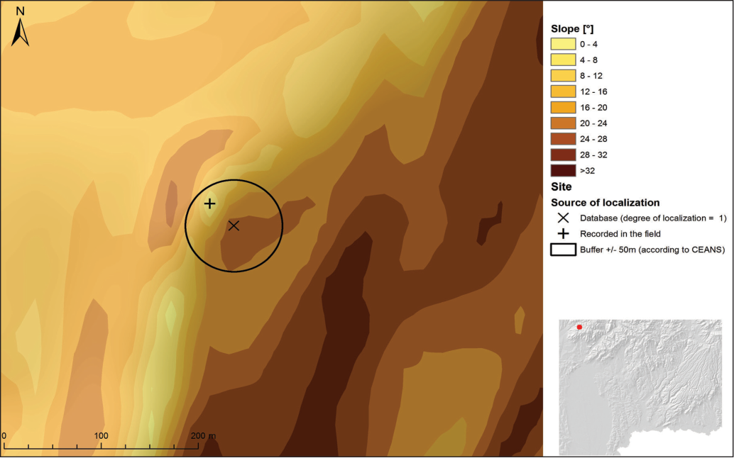
One of the main issues in the application of GIS in archaeology is the geometric positioning of an archaeological site. In the current state of archaeological evidence in Slovakia, accuracy of positioning can be within 100 m, particularly for older and unverified records. This value is based on the rules of the Central Registry of Archaeological Sites in Slovakia (CEANS), where the basic unit of the registration system in the database is a point with a diameter of 4 mm placed on the map with a scale of 1:25,000 which corresponds to 100 m in the field (Bujna et al. 1993). This point from the record of the archaeological sites is a significant source of uncertainty (Figure 5).
This means a generalization towards reality insofar as archaeological sites comprise a large area of polygons. The issue is determining the centroid of a known archaeological site (the core of the site versus the geometric centre) as well as its scope because it is rare that the site is exposed and the entire grounds of the site are known.
Archaeological finds themselves are subject to various transformation processes, deposition processes or spatial movements, such as erosion or soil movements. Similarly, in modelling certain phenomena and the application of theoretical knowledge, human behaviour, which is not always based on rational principles and is characterized by high variability and adaptability, needs to be taken into account. This is reflected in the vagueness of the opinions in the investigation of human history and human behaviour (“proximity to water”, “a suitable slope” and “suitable land”), which are the causes of confusion in the definition of certain standards in spatial analyses. All these facts bring a significant degree of uncertainty and distortion to spatial analyses. Fuzzy logic allows for improved reflecting of the natural estimated properties and modelling of the uncertainty of archaeological spatial data (Lieskovský et al. 2011).
4.2.2 The basic concept of fuzzy sets
The fuzzy set A of a universe X is defined by a membership function mA(x) such that X→〈0,1〉, where mA(x) is the membership value of x in A (Zadeh 1965).
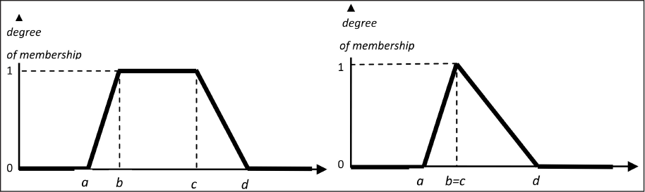
The membership degree reflects the rate to which the element belongs to the set. Fuzzy sets are, therefore, a means providing the ability to mathematically describe vague concepts and work with them. The shape (e.g. the trapezoidal, Gaussian, sinusoidal) and the parameters of the membership functions can be determined on the basis of practical experience or the known properties of the analysed phenomenon. One of the most commonly used functions is the trapezoidal (piecewise linear) membership (Figure 6a) (Kainz 2012): A special case is represented by the triangular membership function (Figure 6b).
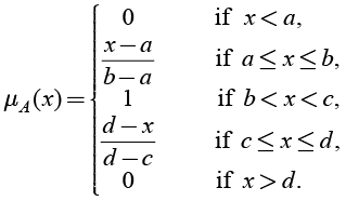 (1)
(1)
A special case is represented by the triangular membership function (Figure 6b).
When creating APM, fuzzy sets were used to model entry criteria (raster data layers) (Lieskovský et al. 2011), (Ďuračiová et al. 2011).
5. The aggregation of layers in the development of APM
Mutual evaluation when meeting individual criteria forms the basis for deciding on the propriety or impropriety of conditions. The process of combining several numerical values into a single representative is known as aggregation and the numerical function performing this process is referred to as the aggregation function. There are three basic classes of aggregation functions: conjunctive functions, disjunctive functions and internal functions. Conjunctive functions combine values as they are related by alogical “and” operator (in fuzzy logic represented by triangular norms). Disjunctive functions combine values as an “or” operator (in fuzzy logic represented by triangular conorms). Internality is a property shared by all the means and averaging functions (Grabisch et al. 2009).
In most cases, the resulting APM, created in the GIS environment, arises either through internal aggregation functions (for example, a weighted arithmetical average) or as a combination of intersections and unions of layers (conjunctive or disjunctive aggregate functions). The work (Lieskovský et al. 2011) describes the basic methods of aggregation of input layers by means of logical operators, such as intersection, union and complementing of the set (AND, OR, NOT). In mathematical logic, these operations correspond to the propositional operations of conjunction, disjunction and negation.
5.1 Fuzzy logic operators
Operations with fuzzy sets also form the basis for the operations of fuzzy propositional calculus but with the truth values coming from the interval 〈0, 1〉 (Navara, Olšák 2002). The operations of the fuzzy conjunction (the intersection of two or more features – criteria), fuzzy disjunction (union), and fuzzy complement (negation) are a generalization of crisp ones. The most widely used operations are known as standard fuzzy set operations (Zadeh 1965):
The intersection (Zadeh 1965) of two fuzzy sets A and B with respective membership functions mA(x) and mB(x) is fuzzy set C, written as C=A∩B, whose membership function is related to those of A and B by
 (2)
(2)
The union (Zadeh 1965) of two fuzzy sets A and B with respective membership functions mA(x) and mB(x) is a fuzzy set C, written as C=A∪B, whose membership function is related to those of A and B by
 (3)
(3)
The complement (Zadeh 1965) of fuzzy set A is denoted by  and is defined by
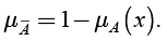 (4)
(4)
The standard complement of fuzzy set A is consequently fuzzy set  with a membership function
  .
.
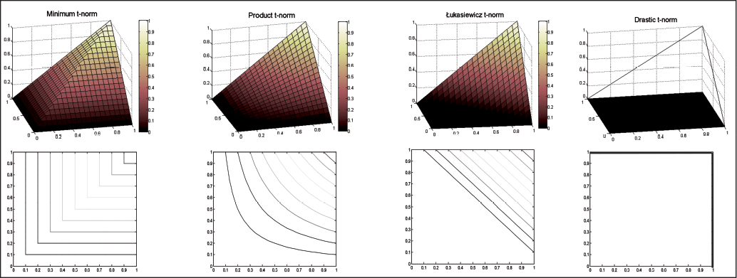
The fuzzy intersection (conjunction) is generally defined by the so-called triangular norms (t-norms) and the fuzzy union (disjunction) using triangular co-norms (t-conorms) (Navara, Olšák 2002). The basic t-norms include (Kolesárová, Kováčová 2004):
 minimum t-norm (Figure 7a) (5)
(standard intersection),
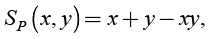
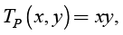 product (Figure 7b), (6)
 Łukasiewicz t-norm (7)
(Figure 7c),
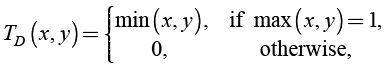 (8)
(8)
drastic t-norm (Figure 7d).
Each t-norm is the aggregate function. The smallest t-norm is TD (x, y) and the greatest is TM (x, y) (Grabisch 2008). The following is valid for basic t-norms:
 (9)
(9)
Corresponding t-conorms are defined as follows (Kolesárová, Kováčová 2004):
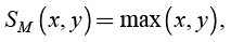 maximum t-conorm (10)
(standard union),
 probabilistic sum, (11)
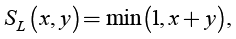 Łukasiewicz t-conorm, (12)
 drastic t-conorm. (13)
5.2 Means and averages
According to (Klir, Yuan 1995), the quasiarithemtic average hl (Generalized means) as the aggregation operator is in (Navara, Olšak 2002) defined as:
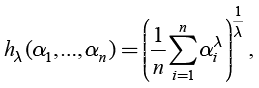 (14)
(14)
where  ,
,  , l ∈ R,
 .
.
Special cases of quasiarithmetic average are:
- • for λ=1 arithmetic average,
- • for λ=2 quadratic average,
- • for λ=–1 harmonic average,
- • for λ=0 geometric average,
- • for λ→+∞ maximum,
- • for λ→–∞ minimum.
The weighted arithmetic average (the weighted linear combination) hw is defined as:
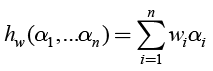 , (15)
where n∈N and  is a vector of weights which fulfils the following condition:
 .
.
The determination of the appropriate weights is often a question of an expert’s judgment or a complex statistical analysis. When creating APM, statistical methods such as basic descriptive statistics, testing statistical distribution, testing rates of disparity and testing cross-correlation of data were even applied to determine the weights of the individual criteria.
An ordered weighted aggregating operator (OWA operator) (Yager 1988)  is also determined by the vector of weights
 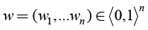 , which satisfy the condition
  (Navara, Olšák 2002):
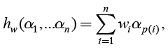 (16)
(16)
where p is a permutation of indices, for which:
 .
.
The minimum, the maximum and the arithmetic average are special cases of OWA operators.
5.3 The choice of the aggregation operator and its impact on the resulting APM
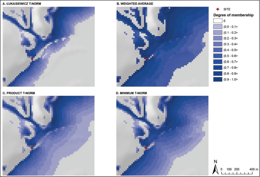
The theory of fuzzy sets defines several fuzzy conjunctions and disjunctions. Their choice for a particular application as well as the choice of any other aggregation operator may significantly influence the outcome. When considering the purpose for which the fuzzy operators are used in spatial analysis, the application of this paper uses the minimum (standard), product and Łukasiewicz conjunction. From the internal aggregation operators’ group we applied the weighted arithmetic average providing, however, non-zero values for each entry decision criterion in order to maintain the exclusive influence of layers on the resulting APM. The selection of the aggregation operator to create APM should result from the nature of the input layers (the decision criteria). Conjunctive aggregate functions, such as a logic operator, intersection and all t-norms are considered to be appropriate operators for the layers of exclusive influence. The general effect of the layers is maintained by the integral aggregate functions (averages). The “attractor” layers are aggregated through disjunctive aggregation functions (the logical operator, the union and all other t-conorms). The “deflector” layers can be included into the model by means of the logical operator of negation.
Figure 8 documents the impact of the choice of the aggregation operators on the resulting APM. The subsequent validation of the APM supports either the propriety or impropriety of their use.
6. Validation of APM
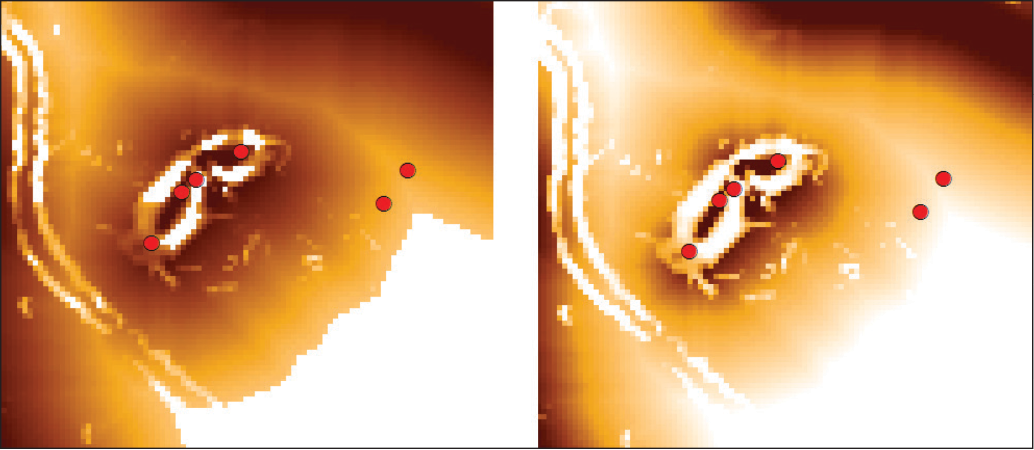
The validation of the model is characterized as a process of its evaluation or, in other words, represents a tool used to determine its quality. Despite the fact that the basic concept of testing (validation) is based on statistics, it is not applicable in most cases of APM statistical testing. Generally, predictive models are the result of the classification process. Moreover, the models work with incomplete data which follow the need to use the specific methods of their testing. Validation of the APM results in the determination of its performance as a degree with which the model correctly and precisely predicts the presence or absence of archaeological sites. Consequently, prior to the actual explanation of each APM validation method, it is important to clarify the meaning of terms such as accuracy and precision of a model, which are closely related to the concepts of gross errors and wasteful errors (errors of the first and the second kind/rate). In predictive modelling, the accuracy of a model is understood as the meaning of a correct prediction signifying whether the model captures the majority of the sites. The model accuracy refers to the ability of a model to limit the areas of occurrence as closely as possible. Since the accuracy and precision combined determine the effectiveness of a model, the quality model should be correct and precise at the same time. Both concepts are well-illustrated in Figure 9.
Gross errors subsequently represent the occurrence of archaeological sites found in zones designated as those of low potential occurrence. The consideration of these errors is assumed in the application of the model for pragmatic purposes, namely to protect the cultural and historical heritage.
Wasteful errors are characterized (Altshul 1988) as the occurrence of “non-sites” situated in the areas designated as those of a high potential occurrence. From the archaeologists’ point of view, wasteful errors constitute a less serious obstacle, although, the model containing a large number of these errors (the model is actually accurate, but is not precise) may lead to higher costs for constructors as long as it will be necessary to carry out archaeological excavation in a larger area than is actually needed.
The risk of committing a gross error is indirectly related to falling into a wasteful error. While the high level of accuracy of the prediction model minimizes gross errors, its high precision minimizes the wasteful ones.
6.1 Basic approaches to the validation of APM
The entire APM validation concept is based on the two following approaches:
1. Internal validation:
The efficiency of the archaeological prediction model is determined from a set of data from which the model was generated. In this case it does not concern new independent collected validation data as the testing process only presents a certain form of internal model validation (internal validation accuracy). This is why the outcome does not provide an adequate answer to the question of the actual efficiency of the prediction model.
2. External validation:
External validation uses validation methods similar to the first case; however, APM is validated on the basis of an independent data sample. Apart from this, the phase also includes a variety of methods for selecting a statistically significant independent data sample. The external form of the test is much more meaningful than the internal validation. The problem of its application is the lack of input data for the database of the archaeological discovery sites in the Slovak Republic.
6.2 Validation methods for archaeological predictive models
The methods for determining the quality of the APM include the calculation of the individual characteristics and the validation parameters. It can be stated in general that the parameter is only suitable for APM validation if it has a value reflecting the quality of the APM and is easily interpretable at the same time (e.g. it takes the values from the interval 〈0, 1〉 where values close to 1 represent an effective model, values close to 0.5 represent the model the prediction level of which is not all that different from random distribution (“a neutral model”) and the lower values correspond to a completely inefficient model).
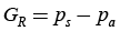
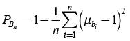
Regarding incomplete archaeological data we utilise the following parameters of APM validation: the statistics gain G (Altschul 1988), the relative statistics gain GR (Altschul 1988), and the effectiveness e (Ďuračiová et al. 2011) and Gini coefficient Gk. The Brier parameter PB (Brier 1950) was modified in order to calculate the validation with incomplete data. The relations for their calculation, as well as the range of values the parameters can take, are shown in Table 2. Figure 10 illustrates the charts of the parameters G, GR and e. The charts also indicate the importance of the e application eliminating the disadvantages of parameters G and GR during validation of APM (Ďuračiová et al. 2011).
The validation methods of APM stated above (apart from the Gini coefficient and Brier’s parameter) are primarily designed for a binary APM (division of the territory into two categories – suitable or unsuitable) or limited by the number of categories of the area propriety (max. 2 – efficiency e). In order to make these methods applicable for validation of fuzzy APM, the individual relations need to be generalized (Karell et al. 2012) or the fuzzy model be transformed for validation purposes using defuzzyfication for the binary model or the model with three categories of suitability (“high suitable area”, mid-suitable area” and “low suitability area”). Defuzzyfication may lead, however, to a reduction in the potential of fuzzy models due to the loss of information about either the suitability or unsuitability of an area.
6.3 The results of APM validation and their evaluation
After creating the models, a complex validation of APM was carried out which was aimed at determining the most appropriate method for APM creation as well as to compare the individual methods’ results from the development and validation of APM. The preliminary results of the model validation were published in the works (Ďuračiová et al. 2011) and (Karell et al. 2012). The course of the external validation results of deductive and inductive-deductive APM for parameters e1–e3, G1–G3, Gk a Pb is shown in Figure 11.
Validation methods were applied to evaluate fuzzy deductive and inductive-deductive APM. As we only had access to data with positive results available from archaeological research, we applied the methods considering this factor. The results for every APM type indicate an evident cross-correlation between the individual parameters and their modifications. Based upon an analysis of the given results and the practical purpose we propose an application of parameter e2 (or G2) which counterbalances the precision and accuracy of the model. Parameter e3 contributes to the relevance of the model’s precision, which is primarily important in terms of the costs for the constructors carrying out the land survey. Parameter Pb evaluates models in terms of their accuracy (a minimization of gross errors) and we thereby consider the protection of the cultural and historical heritage. Since we did not consider the membership level, it is necessary to exclude the parameters e1 (or G1) from the models created by the fuzzy sets (they do not show signs of the difference between the models created by using individual t-norms and those created by means of a weighted arithmetic average). The application of parameter e1 (or G1) still has its meaning in, for instance, deductive-binary APM. The problem of the applied parameters (apart from parameters Gk and Pb) consists in a range of values as the results may take values ±∞ (G only at –∞). This may only be solved by a further modification of the given parameters.
The best results among the fuzzy-deductive and inductive-deductive models were achieved in those APM created by the Łukasiewicz t-norm and the weighted arithmetic average. Significant differences occurred between the models made of layers of fluvial sediments, slope (and perhaps even soil suitability) and the models developed from layers of watercourses, slopes (and soils). This demonstrated that APM consisting of the layer of watercourses reached the significantly lower values of the validation parameters while the contribution of the soils’ layer to increase validation levels is minimal or none (the contribution of this layer is assumed at the availability of higher quality input data).
7. Conclusion
In case of statistical testing of the results of the spatial analysis, it is necessary to determine not only the difference in the distribution of the phenomenon in a country or sites, but also the difference/divergence rate. Given that the impact of the environment influenced the choice of the localities of human activities, the most basic tests (Kolmogorov – Smirnoff test, Chi – square, etc.) demonstrate the impact of these variables on the choice of an area with human activities. Since these tests do not quantify the size of this effect, it is appropriate to use methods quantifying the difference rate and thus potentially establish the importance of each phenomenon. It is additionally possible that the impact of several factors such as the presence of water, the appropriate slope, etc. may through its significance obscure the importance of other factors involved in the decision-making process of selecting the area of human activities. We propose an exploration of the methods which examine the significance of other factors, considering that all dominant factors (trends) have been removed.
The implementation of map algebra operations by an appropriate aggregation function is based on a determination of the impact of layers in a proper way as it is stated in chapter 2 (“Principles of the archaeological predictive models”). The results of the APM analyses’ variants indicated reduced APM accuracy in deductive creating by simplified principles. We recommend applying fuzzy logic instead of a binary one, if possible. The fuzzy sets enable a better expression of the natural assumed characteristics and model the uncertainty of the archaeological and spatial data. The deductive approach is appropriate when there is a sufficient knowledge of the phenomena based on the results of the archaeological research, archaeological theory or sufficient experience. The deductive approach is the only way of modelling in the areas missing information about archaeological localities. We may assume that the data are not statistically relevant (the low, uneven survey of the area of the study). The inductive approach allows us to partially objectify certain statements and assumptions used in the creation of APM as well as determine the importance of individual parameters. By means of the inductive approach we may analyse the changes in the input layers in the case of APM spreading to geographically distinct areas. In contrast, it does not enable a complete model of certain phenomena and is prone to a distortion caused by the uneven survey of the studied area, the accuracy of localization and the indiscrimination of the various types of archaeological localities. The best way is to combine both approaches. When creating a model by the deductive approach using the fuzzy sets, for example, the form of the membership function (chapter 3.2.1) may be adjusted to the basis of the results from the statistical testing of the known parameters and similarly it is then possible to determine the weight of each layer. When applying the mostly inductive approach, the distant and extreme values of the statistical testing can be eliminated on the basis of the deductive assumptions.
The advantage of the inductive-deductive model validation is represented by the similar behaviour of the external validation results for the first and the second sample of the archaeological sites. As expected, the results of the inductive-deductive APM are inferior to the fuzzy deductive APM. We would propose an interest with the optimization process of APM in the future. Possibilities for making them more accurate are based on choosing appropriate membership functions, excluding specific archaeological localities, which do not correspond to the common patterns of a settlement, but refer to the territory being attractive for another reason, e.g. in terms of mining, the cult factor, etc., dividing localities into residential areas and hill-forts, or using a better quality layer of soil types. The modification of APM should improve the results of the inductive-deductive APM validation.
Spatial archaeology and predictive modelling as its application are important elements of the archaeological research and clarify the relationship between humans and the landscape. Their development was enabled by the arrival of new theoretical approaches and paradigms. The combination of GIS and spatial archaeology allows for modelling and verifying the archaeological theories and assumptions and represents an effective method of cultural-historical heritage protection.
Archaeological predictive modelling is an interesting problem in terms of geoinformatics, mathematics and statistics. Although the degree of understanding is continually increasing, as well as the amount of applicable spatial data, the quality and quantity of archaeological data, the possibilities of historical environment reconstruction and ultimately the state of the art are still limiting factors in APM creation. These limits are typical for other natural sciences as well and there is a need to know the processing capabilities and develop new solutions and methods, which would be applicable in the sphere of archaeology and elsewhere.
Acknowledgements
This work was supported by the Slovak Research and Development Agency under contract No. APVV-0249-07.
References
ALTSCHUL, J. H. 1988: Quantifying the present and predicting the past: Theory, Method, and Application of Archeological Predictive Modeling. U.S. Department of the Interior, Bureau of Land Management Service Center Denver, Colorado.
BRIER, G. W. 1950: Verification of forecasts expressed in terms of probability. U.S. Weather Bureau, Washington, D.C.
BUJNA, J. et al. 1993: CEANS – Centrálna evidencia archeologických nálezísk na Slovensku – Projekt systému. Slovenská archeológia XLI 2, 367–386.
DANIELISOVÁ, A. 2008: Oppidium České Lhotice v kontextu svého sídelního zázemí. (The oppidum of České Lhotice and its hinterland). MS. Thesis. Deposited: Charles University, Faculty of Arts, Prague.
ĎURAČIOVÁ, R., LIESKOVSKÝ, T., KROČKOVÁ, K., SABO, M. 2011: Multikriteriálne rozhodovanie pomocou fuzzy množín v prostredí GIS a jeho využitie v archeologickej predikcii. Geodetický a kartografický obzor 09/2011, 205–217.
GRABISCH, M., MARICHAL, J.-L., MESIAR, R., PAP, E. 2009: Aggregation Functions, Encyclopedia of Mathematics and its Applications, No 127. Cambridge University Press, Cambridge.
GOLÁŇ, J. 2003: Archeologické prediktivní modelovaní pomocí geografických informačních systémů: Na příkladu území jihovýchodní Moravy. MS. Thesis. Deposited: Masaryk University, Faculty of Science, Brno.
KAINZ, W. 2012: Fuzzy Logic and GIS, on-line: http://www.scribd.com/doc/44096805/Fuzzy-in-GIS-Basic (accessed in June 2012).
KARELL, L., LIESKOVSKÝ, T., ĎURAČIOVÁ, R. 2012: Validácia archeologických predikčných modelov vytvorených pomocou fuzzy množín v prostredí GIS. Kartografické listy/ Cartographic letters, 20 (2), 25–35.
KLIR, G. J., YUAN, B. 1995: Fuzzy Sets and Fuzzy Logic. Theory and Applications. Prentice-Hall.
KOLESÁROVÁ, A., KOVÁČOVÁ, M. 2004: Fuzzy množiny a ich aplikácie. Slovak University of Technology in Bratislava, Bratislava.
LEUSEN, M. et al. 2005: A baseline for Predictive Modelling in the Netherlands. Amersfoort.
LIESKOVSKÝ, T. 2011: Využitie geografických informačných systémov v predikčnom modelovaní v archeológii. MS. Disertation thesis, Deposited: Slovak University of Technology in Bratislava, Faculty of Civil Engineering, Bratislava.
LIESKOVSKÝ, T., FAIXOVÁ CHALACHANOVÁ, J., ĎURAČIOVÁ, R., BLAŽOVÁ, E. 2011: Archeologické predikčné modelovanie z pohľadu geoinformatiky. REMPrint, s.r.o., Bratislava.
NAVARA, M., OLŠÁK, P. 2002: Základy fuzzy množín. Vydavatelství ČVUT, Praha.
NEUSTUPNÝ, E. 2007: Metoda archeologie. Aleš Čeněk, Plzeň.
YAGER, R. R. 1988: On Ordered Weighted Averaging Aggregation Operators in Multicriteria
Decision making, IEEE Trans’ on Systems’. Man and Cybernetics 18, 183–190.
ZADEH, L. 1965: Fuzzy Sets. Information and Control 8, 338–353.